Getting started
This tutorial highlights the basics of the high-level API for ensemble classes, the model selection suite and features visualization.
| Tutorials | Content |
|---|---|
| Ensemble guide | How to build, fit and predict with an ensemble |
| Model selection guide | How to compare several estimators in one go |
| Visualization guide | Plotting functionality |
The advanced high-level API tutorials shows how to leverage advanced features such as probabilistic layers, feature propagation etc. For tutorials on low-level mechanics, see the mechanics guides.
Preliminaries
We use the following setup throughout:
import numpy as np
from pandas import DataFrame
from sklearn.metrics import accuracy_score
from sklearn.datasets import load_iris

seed = 2017
np.random.seed(seed)

data = load_iris()
idx = np.random.permutation(150)
X = data.data[idx]
y = data.target[idx]
Ensemble guide
Building an ensemble
Instantiating a fully specified ensemble is straightforward and requires three steps: first create the instance, second add the intermediate layers, and finally the meta estimator.
from mlens.ensemble import SuperLearner
from sklearn.linear_model import LogisticRegression
from sklearn.ensemble import RandomForestClassifier
from sklearn.svm import SVC

# --- Build ---
# Passing a scoring function will create cv scores during fitting
# the scorer should be a simple function accepting to vectors and returning a scalar
ensemble = SuperLearner(scorer=accuracy_score, random_state=seed, verbose=2)

# Build the first layer
ensemble.add([RandomForestClassifier(random_state=seed), SVC()])

# Attach the final meta estimator
ensemble.add_meta(LogisticRegression())

# --- Use ---

# Fit ensemble
ensemble.fit(X[:75], y[:75])

# Predict
preds = ensemble.predict(X[75:])
Out:
Fitting 2 layers
Processing layer-1             done | 00:00:00
Processing layer-2             done | 00:00:00
Fit complete                        | 00:00:00

Predicting 2 layers
Processing layer-1             done | 00:00:00
Processing layer-2             done | 00:00:00
Predict complete                    | 00:00:00
To check the performance of estimator in the layers, call the data
attribute. The attribute can be wrapped in a pandas.DataFrame,
but prints in a tabular format as is.
print("Fit data:\n%r" % ensemble.data)
Out:
Fit data:
                                   score-m  score-s  ft-m  ft-s  pt-m  pt-s
layer-1  randomforestclassifier       0.84     0.06  0.05  0.00  0.00  0.00
layer-1  svc                          0.89     0.05  0.01  0.00  0.00  0.00
To round off, let’s see how the ensemble as a whole fared.
print("Prediction score: %.3f" % accuracy_score(preds, y[75:]))
Out:
Prediction score: 0.960
Multi-layer ensembles
With each call to the add method, another layer is added to the ensemble.
Note that all ensembles are sequential in the order layers are added. For
instance, in the above example, we could add a second layer as follows.
ensemble = SuperLearner(scorer=accuracy_score, random_state=seed)

# Build the first layer
ensemble.add([RandomForestClassifier(random_state=seed), LogisticRegression()])

# Build the second layer
ensemble.add([LogisticRegression(), SVC()])

# Attach the final meta estimator
ensemble.add_meta(SVC())
We now fit this ensemble in the same manner as before:
ensemble.fit(X[:75], y[:75])
preds = ensemble.predict(X[75:])
print("Fit data:\n%r" % ensemble.data)
Out:
Fit data:
                                   score-m  score-s  ft-m  ft-s  pt-m  pt-s
layer-1  logisticregression           0.75     0.14  0.01  0.01  0.00  0.00
layer-1  randomforestclassifier       0.84     0.06  0.03  0.00  0.00  0.00
layer-2  logisticregression           0.67     0.12  0.01  0.00  0.00  0.00
layer-2  svc                          0.89     0.00  0.00  0.00  0.00  0.00
Model selection guide
The work horse class is the Evaluator, which allows you to
grid search several models in one go across several preprocessing pipelines.
The evaluator class pre-fits transformers, thus avoiding fitting the same
preprocessing pipelines on the same data repeatedly. Also, by fitting all
models over all parameter draws in one operation, parallelization is
maximized.
The following example evaluates a Naive Bayes estimator and a
K-Nearest-Neighbor estimator under three different preprocessing scenarios:
no preprocessing, standard scaling, and subset selection.
In the latter case, preprocessing is constituted by selecting a subset of
features.
The scoring function
An important note is that the scoring function must be wrapped by
make_scorer(), to ensure all scoring functions behave similarly regardless
of whether they measure accuracy or errors. To wrap a function, simple do:
from mlens.metrics import make_scorer
accuracy_scorer = make_scorer(accuracy_score, greater_is_better=True)
The make_scorer wrapper
is a copy of the Scikit-learn’s sklearn.metrics.make_scorer(), and you
can import the Scikit-learn version as well.
Note however that to pickle the Evaluator, you must import
make_scorer from mlens.
A simple evaluation
Before throwing preprocessing into the mix, let’s see how to evaluate a set of
estimator. First, we need a list of estimator and a dictionary of parameter
distributions that maps to each estimator. The estimators should be put in a
list, either as is or as a named tuple ((name, est)). If you don’t name
the estimator, the Evaluator will automatically name the model as the
class name in lower case. This name must be the key in the parameter
dictionary.
from mlens.model_selection import Evaluator
from sklearn.naive_bayes import GaussianNB
from sklearn.neighbors import KNeighborsClassifier
from scipy.stats import randint

# Here we name the estimators ourselves
ests = [('gnb', GaussianNB()), ('knn', KNeighborsClassifier())]

# Now we map parameters to these
# The gnb doesn't have any parameters so we can skip it
pars = {'n_neighbors': randint(2, 20)}
params = {'knn': pars}
We can now run an evaluation over these estimators and parameter distributions
by calling the fit method.
evaluator = Evaluator(accuracy_scorer, cv=10, random_state=seed, verbose=1)
evaluator.fit(X, y, ests, params, n_iter=10)
Out:
Launching job
Job           done | 00:00:00
The full history of the evaluation can be found in cv_results. To compare
models with their best parameters, we can pass the results attribute to
a pandas.DataFrame or print it as a table. We use m to denote
mean values and s to denote standard deviation across folds for brevity.
Note that the timed prediction is for the training set, for comparability with
training time.
print("Score comparison with best params founds:\n\n%r" % evaluator.results)
Out:
Score comparison with best params founds:

       test_score-m  test_score-s  train_score-m  train_score-s  fit_time-m  fit_time-s  pred_time-m  pred_time-s               params
gnb           0.960         0.033          0.957          0.006       0.006       0.002        0.004        0.002
knn           0.967         0.033          0.980          0.005       0.002       0.001        0.010        0.004  {'n_neighbors': 15}
Preprocessing
Next, suppose we want to compare the models across a set of preprocessing pipelines. To do this, we first need to specify a dictionary of preprocessing pipelines to run through. Each entry in the dictionary should be a list of transformers to apply sequentially.
from mlens.preprocessing import Subset
from sklearn.preprocessing import StandardScaler

# Map preprocessing cases through a dictionary
preprocess_cases = {'none': [],
                    'sc': [StandardScaler()],
                    'sub': [Subset([0, 1])]
                    }
The fit methods determines automatically whether there is any preprocessing
or any estimator jobs to run, so all we need to do is specify the arguments
we want to be processed. If a previous preprocessing job was fitted, those
pipelines are stored and will be used for subsequent estimator fits.
This can be helpful if the preprocessing is time-consuming, for instance if
the preprocessing pipeline is an ensemble itself. All ensembles implement
a transform method that, in contrast to the predict method, regenerates
the predictions made during the fit``call. More precisely, the ``transform
method uses the estimators fitted with cross-validation to construct predictions,
whereas the predict method uses the final estimators fitted on all data.
This allows us use ensembles as preprocessing steps that mimicks how that ensemble
would produce predictions for a subsequent meta learner or layer. Since fitting
large ensembles is highly time-consuming, fixing the lower layers as preprocessing
input is highly valuable for tuning the higher layers and / or the final meta learner.
See the Ensemble model selection tutorial for
an example. To fit only the preprocessing pipelines, we omit any estimators in the
fit call.
evaluator.fit(X, y, preprocessing=preprocess_cases)
Out:
Launching job
Job           done | 00:00:00
Model Selection across preprocessing pipelines
To evaluate the same set of estimators across all pipelines with the same parameter distributions, there is no need to take any heed of the preprocessing pipeline, just carry on as in the simple case:
evaluator.fit(X, y, ests, params, n_iter=10)
print("\nComparison across preprocessing pipelines:\n\n%r" % evaluator.results)
Out:
Launching job
Job           done | 00:00:01

Comparison across preprocessing pipelines:

             test_score-m  test_score-s  train_score-m  train_score-s  fit_time-m  fit_time-s  pred_time-m  pred_time-s               params
none  gnb           0.960         0.033          0.957          0.006       0.004       0.001        0.003        0.001
none  knn           0.967         0.033          0.980          0.005       0.002       0.001        0.006        0.001  {'n_neighbors': 15}
sc    gnb           0.960         0.033          0.957          0.006       0.004       0.001        0.003        0.001
sc    knn           0.960         0.044          0.965          0.003       0.001       0.001        0.006        0.001   {'n_neighbors': 8}
sub   gnb           0.780         0.133          0.791          0.020       0.004       0.001        0.004        0.001
sub   knn           0.800         0.126          0.837          0.015       0.002       0.001        0.005        0.002   {'n_neighbors': 9}
You can also map different estimators to different preprocessing folds, and map different parameter distribution to each case. We will map two different parameter distributions
pars_1 = {'n_neighbors': randint(20, 30)}
pars_2 = {'n_neighbors': randint(2, 10)}
params = {'sc.knn': pars_1,
          'none.knn': pars_2,
          'sub.knn': pars_2}

# We can map different estimators to different cases
ests_1 = [('gnb', GaussianNB()), ('knn', KNeighborsClassifier())]
ests_2 = [('knn', KNeighborsClassifier())]
estimators = {'sc': ests_1,
              'none': ests_2,
              'sub': ests_1}

evaluator.fit(X, y, estimators, params, n_iter=10)
print("\nComparison with different parameter dists:\n\n%r" % evaluator.results)
Out:
Launching job
Job           done | 00:00:01

Comparison with different parameter dists:

             test_score-m  test_score-s  train_score-m  train_score-s  fit_time-m  fit_time-s  pred_time-m  pred_time-s               params
none  knn           0.967         0.045          0.961          0.007       0.002       0.001        0.003        0.001   {'n_neighbors': 3}
sc    gnb           0.960         0.033          0.957          0.006       0.004       0.001        0.002        0.001
sc    knn           0.940         0.055          0.959          0.008       0.002       0.000        0.008        0.001  {'n_neighbors': 22}
sub   gnb           0.780         0.133          0.791          0.020       0.003       0.001        0.003        0.001
sub   knn           0.800         0.126          0.837          0.015       0.002       0.001        0.004        0.002   {'n_neighbors': 9}
Visualization guide
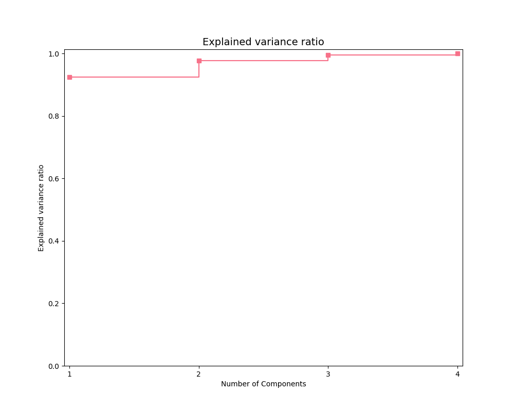
Explained variance plot
The exp_var_plot function
plots the explained variance from mapping a matrix X onto a smaller
dimension using a user-supplied transformer, such as the Scikit-learn
sklearn.decomposition.PCA transformer for
Principal Components Analysis.
import matplotlib.pyplot as plt
from mlens.visualization import exp_var_plot
from sklearn.decomposition import PCA
exp_var_plot(X, PCA(), marker='s', where='post')
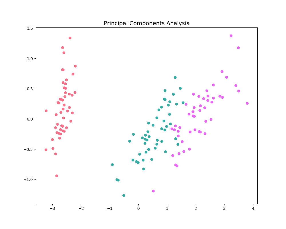
Principal Components Analysis plot
The pca_plot function
plots a PCA analysis or similar if n_components is one of [1, 2, 3].
By passing a class labels, the plot shows how well separated different classes
are.
from mlens.visualization import pca_plot
from sklearn.decomposition import PCA
pca_plot(X, PCA(n_components=2), y=y)
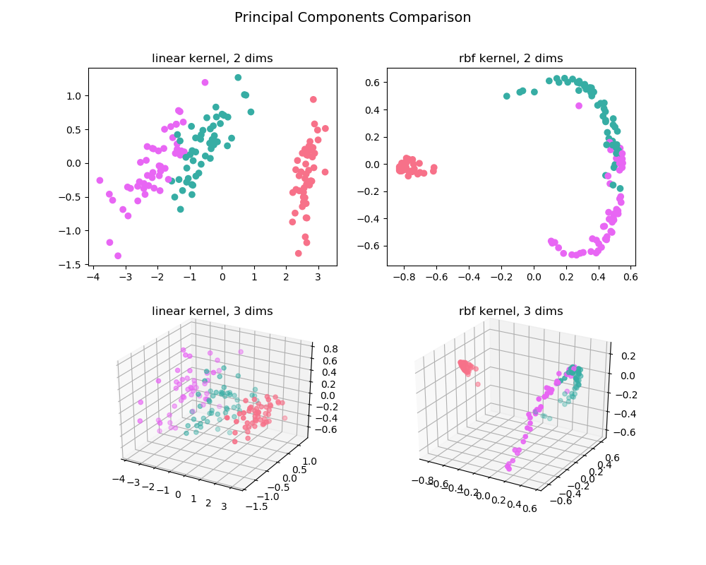
Principal Components Comparison plot
The pca_comp_plot function
plots a matrix of PCA analyses, one for each combination of
n_components=2, 3 and kernel='linear', 'rbf'.
from mlens.visualization import pca_comp_plot
pca_comp_plot(X, y)
plt.show()
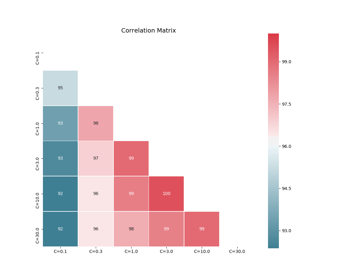
Correlation matrix plot
The corrmat function plots the lower triangle of
a correlation matrix and is adapted the Seaborn correlation matrix.
from mlens.visualization import corrmat
# Generate som different predictions to correlate
params = [0.1, 0.3, 1.0, 3.0, 10, 30]
preds = np.zeros((150, 6))
for i, c in enumerate(params):
    preds[:, i] = LogisticRegression(C=c).fit(X, y).predict(X)

corr = DataFrame(preds, columns=['C=%.1f' % i for i in params]).corr()
corrmat(corr)
plt.show()
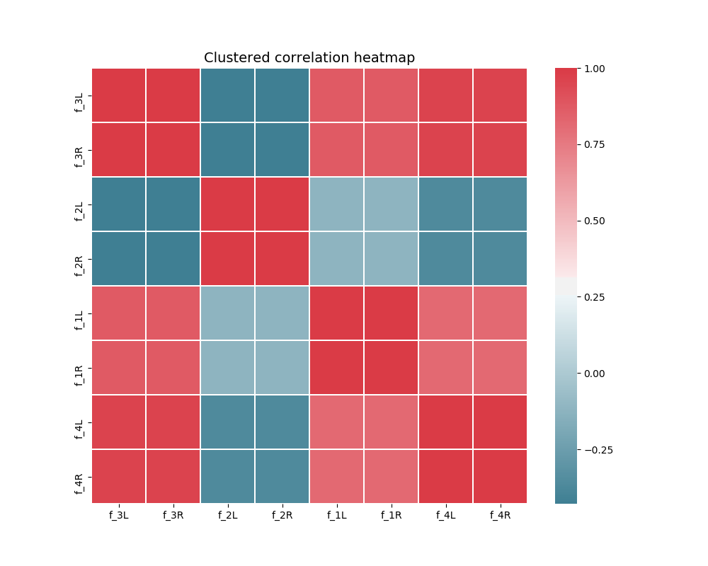
Clustered correlation heatmap plot
The clustered_corrmap function is similar to corrmat,
but differs in two respects. First, and most importantly, it uses a user
supplied clustering estimator to cluster the correlation matrix on similar
features, which can often help visualize whether there are blocks of highly
correlated features. Secondly, it plots the full matrix (as opposed to the
lower triangle).
from mlens.visualization import clustered_corrmap
from sklearn.cluster import KMeans
Z = DataFrame(X, columns=['f_%i' % i for i in range(1, 5)])
We duplicate all features, note that the heatmap orders features as duplicate pairs, and thus fully pick up on this duplication.
corr = Z.join(Z, lsuffix='L', rsuffix='R').corr()
clustered_corrmap(corr, KMeans())
plt.show()
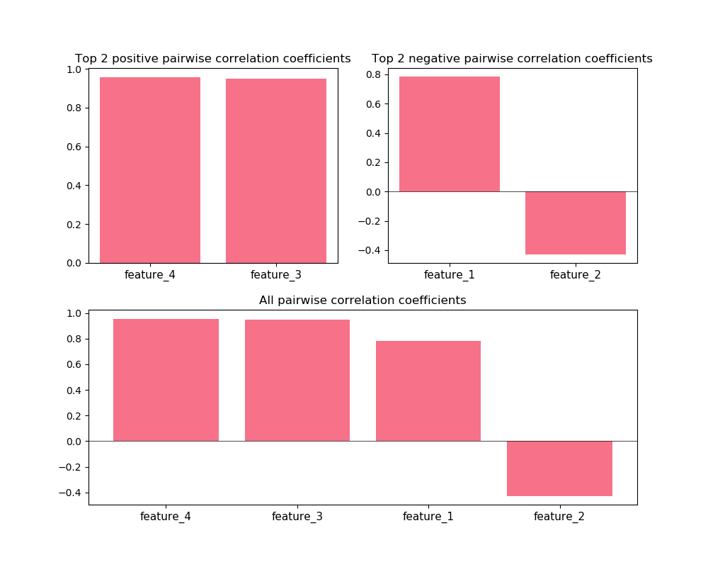
Input-Output correlations
The corr_X_y function gives a dashboard of
pairwise correlations between the input data (X) and the labels to be
predicted (y). If the number of features is large, it is advised to set
the no_ticks parameter to True, to avoid rendering an illegible
x-axis. Note that X must be a pandas.DataFrame.
from mlens.visualization import corr_X_y
Z = DataFrame(X, columns=['feature_%i' % i for i in range(1, 5)])
corr_X_y(Z, y, 2, no_ticks=False)
plt.show()
Total running time of the script: ( 0 minutes 5.928 seconds)